Blog

Your blog category

How to Calculate EMI in Excel

Are you planning a loan or teaching finance? Understanding how to calculate EMI (Equated Monthly Installment) using Microsoft Excel is a must-have skill. Whether it’s a home loan, personal loan, or education loan, Excel makes it simple and quick. In this blog post, we’ll walk you through how to calculate EMI using Excel’s PMT function — with examples and formulas. 💡 What is EMI? EMI stands for Equated Monthly Installment. It’s a fixed monthly payment made by a borrower to a lender. It consists of two parts: Principal – the original loan amount Interest – the cost of borrowing the money 📘 EMI Formula in Excel To calculate EMI in Excel, we use the PMT function: excel CopyEdit =PMT(rate, nper, pv) Where: rate = interest rate per period (monthly interest) nper = total number of payments (loan tenure in months) pv = present value or loan amount 🧠 Example: Let’s say: Loan Amount (Principal) = ₹5,00,000 Annual Interest Rate = 10% Tenure = 5 years (60 months) In Excel: matlab CopyEdit =PMT(10%/12, 60, -500000) Result: ₹10,624.67(This is your monthly EMI) 👉 Note: We use a negative sign before the principal (-500000) to get a positive EMI output. 📊 Bonus: Create a Mini EMI Calculator in Excel   A B Loan Amount 500000 Annual Interest Rate 10% Loan Tenure (in years) 5 Monthly EMI =PMT(B3/12, B4*12, -B2) You can now change the values in column B and see the EMI update instantly. 🎯 Why Learn This? ✅ Helps in financial planning ✅ Essential for finance & accounting professionals ✅ Useful for personal budgeting and client advisory ✅ Frequently asked in interviews & assessments 📌 Final Tip You can also use Excel to break down the EMI into Principal & Interest components, create amortization schedules, and even visualize loan repayments using charts. 📚 Learn More with VertiSkills Want to master Excel for accounting and finance?Join our Advanced Excel Course – packed with real-life projects, functions, and job-oriented training. 📅 New Batch Starting Soon!📞 Contact us at [Your Phone Number] | 🌐 Visit: www.vertiskills.com Let me know if you’d like a downloadable Excel template or images for this blog!

How to Calculate EMI in Excel Read More »

How to Convert Date to Month in Excel

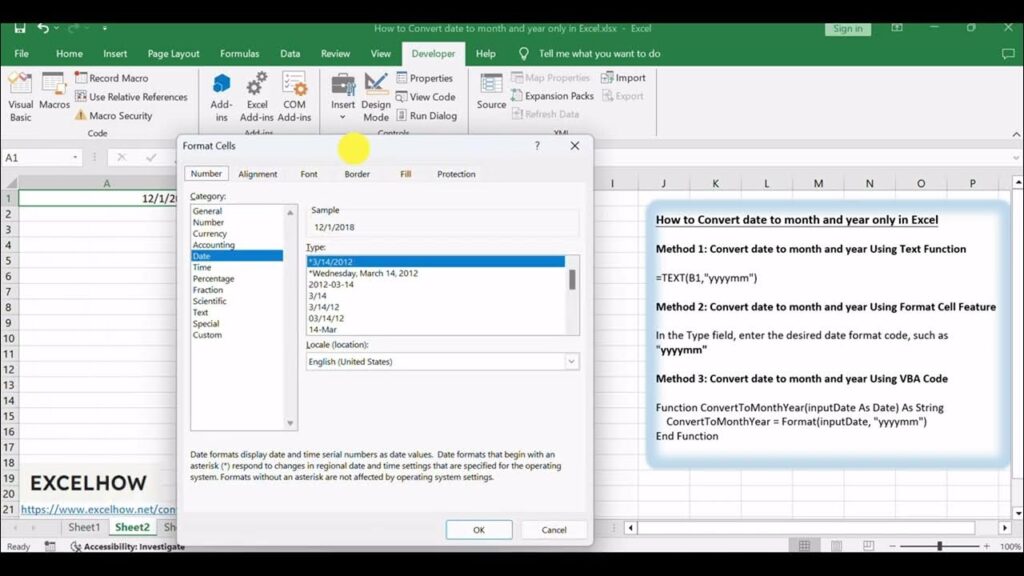
Transforming dates into months in Excel is a handy skill for professionals, as it significantly improves data analysis and visualization. Converting specific dates to months makes it much simpler to spot trends, patterns, and changes over time. According to Acuity Training, Excel is used at least once an hour by two-thirds of office workers (66%). All in all, this feature boosts the accuracy and effectiveness of data analysis in Excel, empowering professionals to make informed decisions based on well-organized and timely data. Here in this article, we have discussed how to convert date to month in Excel. So, let’s get started. Understanding Dates In Excel In Excel, date functions are essential for efficiently handling various data analysis and reporting tasks. Functions like TODAY(), WEEKDAY(), and EOMONTH() allow users to manipulate data values, helping to create insightful reports and analyses. Plus, Excel provides a plethora of formatting options to tailor the appearance of dates in cells. You can easily switch formats from MM/DD/YYYY to DD/MM/YYYY or even apply custom date formats to meet specific needs. These formatting choices not only boost the readability of your data but also help present information in a more visually appealing way. By grasping and using these date functions and formatting options in Excel, you can greatly enhance the accuracy and efficiency of data management and analysis in professional environments. Converting Date To Month Using The TEXT Function Converting dates to months might sound straightforward, but typing out each month by hand can eat up your time and lead to mistakes. That’s why the TEXT function is such a lifesaver! With just a few easy steps, you can quickly transform dates into months in Excel using this handy function. Step 1: Open your Excel spreadsheet and locate the cell where you want to display the month. Step 2: Enter the following formula into the cell where you want to display the month: =TEXT(A1, “mmmm”) Step 3: Replace “A1” in the formula with the cell reference where the date you want to convert is located. Step 4: Press Enter. The cell will now display the month corresponding to the date in the original cell. For example, if cell A1 contains the date “01/15/2022,” entering the formula =TEXT(A1, “mmmm”) in another cell will display “January.” You can also customize the format of the month display by changing the “mmmm” in the formula to “mmm” for a three-letter abbreviation of the month, or “mm” for a two-digit representation of the month. Converting Date to Month Using the MONTH Function One of the great features in Excel is the MONTH function, which makes it super easy to pull the month out of a date in a cell. In this step-by-step guide, we’ll take you through the process of extracting the month from a date using this useful function. Step 1: Open your Excel spreadsheet and locate the cell containing the date from which you want to extract the month. Step 2: Click on the cell where you want the month value to appear. This is where the result of the MONTH function will be displayed. Step 3: Type the following formula into the cell: =MONTH(cell reference). Replace “cell reference” with the cell containing the date you want to extract the month from. For example, if your date is in cell A1, the formula should look like this: =MONTH(A1). Step 4: Press Enter on your keyboard to apply the formula. The cell will now display the numerical representation of the month (1 for January, 2 for February, and so on). Step 5: If you want the month to be displayed as the name of the month rather than a number, you can use the TEXT function in conjunction with the MONTH function. To do this, type the following formula into the cell: =TEXT(MONTH(cell reference), “mmmm”). Again, replace “cell reference” with the cell containing the date. For example, if your date is in cell A1, the formula should look like this: =TEXT(MONTH(A1), “mmmm”). Step 6: Press Enter on your keyboard to apply the formula. The cell will now display the name of the month instead of a number. Using Pivot Tables And Charts For Analysis Converted dates are super important when it comes to pivot tables and charts for data analysis. They give us a consistent format that makes it easy to group, filter, and sort information that’s tied to specific times. By changing dates into a standard format like YYYY-MM-DD, users can dive into trends and patterns over time. In pivot tables, these converted dates can help create calculated fields or items that summarize data for certain date ranges, giving us deeper insights into performance metrics or sales figures. Plus, in charts, converted dates can serve as x-axis values, helping us visualize changes over time and spot connections between different variables. The versatility of converted dates in pivot tables and charts makes data analysis much more thorough and helps professionals make smart decisions based on solid, reliable information. Wrap-Up On How To Convert Date To Month In Excel Mastering the art of converting dates to months in Excel is an essential skill for data analysts. It helps them organize and analyze time-based data more effectively. When analysts convert dates into months, they can spot trends, patterns, and anomalies across various time frames, which is crucial for making informed business decisions. This technique also makes it easier to visualize data through graphs and charts, allowing for clearer communication of findings to stakeholders. Plus, by converting dates to months, analysts can streamline their work, cutting down on manual tasks and ensuring their calculations are spot on. We hope this comprehensive guide has helped you to convert date to month in Excel. If you still have any questions or doubts regarding this article, please let us know in the comments below.

How to Convert Date to Month in Excel Read More »

How to Open a JSON File in Excel

Opening JSON files in Excel makes data analysis and visualization a breeze. JSON, which stands for JavaScript Object Notation, is a widely used format for storing and sharing data because it’s lightweight and easy for humans to read. According to microbizmag. Google Suite features are used by an astounding 2 billion individuals every month.  When you open JSON files in Excel, you can effortlessly transform that structured data into a table format that works seamlessly with Excel’s features like sorting, filtering, and creating charts. This means you can manipulate your data quickly and efficiently, without having to dive into complicated coding or rely on specialized software. Here in this article, we have discussed how to open a JSON file in Excel. So, let’s get started. Understanding JSON Files JSON, or JavaScript Object Notation, is a simple and lightweight format for exchanging data that’s super easy for people to read and write, as well as for machines to process. These files are made up of key-value pairs nestled within curly brackets, which makes them perfect for organizing structured data. When it comes to data analysis, JSON files play a vital role because they offer a consistent way to share data between different systems, allowing for smooth interoperability across various platforms and programming languages. JSON files make it easier to extract, manipulate, and visualize data sets for analysis. Using JSON in data analysis helps analysts manage large amounts of diverse data efficiently and accurately, leading to insights that support smart decision-making in professional environments. Methods of Opening JSON Files in Excel When you want to open JSON files in Excel, there are a few different ways professionals can tackle this task effectively. Ultimately, the method you choose will hinge on the specific needs of your project and your level of expertise. Method 1: Using the Power Query Editor In the realm of data analysis, having the ability to import and work with data from different sources is an essential skill. JSON files are widely utilized for storing and sharing data, and knowing how to bring them into Power Query Editor can unlock a treasure trove of opportunities for your data analysis projects. In this article, we’ll guide you through the steps to import a JSON file using Power Query Editor. Step 1: Launch Power Query Editor To begin the process of importing a JSON file into Power Query Editor, you will first need to launch the program. You can do this by opening Microsoft Excel and selecting the “Data” tab from the ribbon. From there, click on the “Get Data” option and choose “From File.” Then, select “From JSON.” Step 2: Select the JSON file Once you have chosen the “From JSON” option, you will need to navigate to the location of the JSON file that you want to import. Select the file and click “Import.” Step 3: Transform And Load The Data After importing the JSON file, Power Query Editor will display the data in a tabular format. From here, you can apply various transformations to the data to clean it up and prepare it for analysis. This may include removing columns, renaming headers, converting data types, and more. Step 4: Load The Data Into Excel Once you have finished transforming the data, you can click on the “Close & Load” button to load the data into Excel. This will create a new table in your Excel worksheet that contains the imported JSON data. Method 2: Using An Online Converter Tool There are online tools that make it super easy to convert JSON files to Excel format in just a few straightforward steps. we’ll guide you through the process of converting JSON to Excel using one of these handy online tools. Step 1: Choose An Online Tool There are several online tools available for converting JSON to Excel. Some popular options include are aspose, and conversion tools. Choose the tool that best fits your needs and preferences. Step 2: Upload Your JSON File Once you have selected an online tool, you will need to upload your JSON file. Most tools have a user-friendly interface that allows you to easily upload your file. Simply click on the “Upload” button and select the JSON file from your computer. Step 3: Map the JSON Data After uploading your JSON file, the online tool will prompt you to map the data fields. This step is crucial for accurately converting the JSON data to Excel format. The tool will provide you with options to select the fields you want to include in the Excel file. Step 4: Convert to Excel Once you have mapped the JSON data fields, you can proceed to convert the file to Excel format. Click on the “Convert” or “Download Excel” button, depending on the specific tool you are using. The online tool will generate an Excel file containing your JSON data in a tabular format. Step 5: Download and Save the Excel File Finally, download and save the Excel file to your computer. You can now open the file in Microsoft Excel or any other spreadsheet software of your choice. You can further manipulate and analyze the data using Excel’s powerful features. Tips And Tricks For Working With JSON Data In Excel Cleaning up and organizing data in JSON format is super important for getting accurate results in data analysis. When researchers take the time to eliminate inconsistencies, errors, or duplicates from their datasets, they can be confident that their analyses are grounded in trustworthy information. This process includes spotting and fixing any formatting problems, like missing values or incorrect data types, to keep the data’s integrity intact. Once everything is cleaned up and neatly organized, diving into data analysis becomes a lot smoother and more effective. By using techniques like filtering, sorting, and visualizing the JSON data, researchers can uncover valuable insights and patterns that help guide their decision-making.  Wrap-Up On How To Open A JSON File In Excel In the world of data analysis, knowing how to work

How to Open a JSON File in Excel Read More »